Alabama combined temperatures

There are fifteen USHCN stations in Alabama that start at Brewton and end at Valley Head. It has two GISS stations on the list, and they are at Mobile and Montgomery.

USHCN stations in Alabama (CDIAC )

The station in Montgomery is yet another where GISS is using a station that does not start its record until 1947. It is interesting to see how many times GISS is using these shorter truncated records when there are a significant number of other stations that have a full record back into the 1880’s. If one were cynical one might think that this was to hide the higher temperatures in the 1930’s.

Average annual temperatures for Montgomery AL, GISS station data

However there wasn’t such a temperature high in the ‘30’s, for Mobile, whose temperatures have remained relatively stable, so we’ll have to see if there was one for the state as a whole.

Average annual temperatures for Mobile AL, GISS station data

When looking at the difference between the average GISS and the average of the homogenized data for the USHCN sites for this state, the GISS sites are, on average 3 deg F warmer, but there is no trend in the data for Alabama.

Difference in average temperature, per year, between the GISS stations and the homogenized values for the USHCN stations in Alabama.

In terms of the temperature trend for the state, as a whole, even the homogenized data from the USHCN sites shows that the state has cooled over the last century.

Average temperature for the state of Alabama with time, using the homogenized temperature data from the USHCN.

When this is compared with the Time of Observation adjusted raw data (TOBS), that also shows a decline. It is interesting that in both there is a drop in the average temperature in 1958, which then seems to re-stabilize around a lower temperature

Average temperature for the state of Alabama with time, using the Time of Observation corrected raw temperature data from the USHCN.

Looking at the populations surrounding the different stations, using the citi-data sites for the communities, This does not work for Gainsville, which has a population of 192 according to HomeTownLocator. Saint Bernard is a little more of a challenge – so I go to Google Earth, and while close in it looks very rural (being in a Benedictine monastery/school) when one zooms out a little it is in the community of Cullman, AL).

Location of the station at Saint Bernard AL, Cullman is over the hill to the left.

Alabama is some 330 miles long and 190 miles wide, stretching from just under 85 deg N to just under 88.5 deg N, and from 30.21 deg W to 35 deg W. The mean latitude is at 32.84 deg N, that of the USHCN stations is 32.8 deg N, and that of the GISS stations is at 31.5 deg N. The elevation ranges from sea-level to 733 m, with a mean elevation of 152.4 m. The mean elevation of the USHCN network is at 122 m, while that of the GISS stations is 40.5 m. The two GISS stations have an average population of 197,648, while that of the USHCN is 14,866. (With a temperature change of 0.024 deg per m, the change in elevation gives a 1.6 degree difference because of elevation changes, and using a temp change that varies with 0.6 x log (pop) would explain another 0.7 degrees of the average 3.04 deg between the two mean temperatures).

Looking at the effects of state geography on temperature change, beginning with Latitude.

Average Alabama temperature as a function of latitude

Alabama is another state where there is a fall in elevation moving West, and so there is a temperature increase with longitude:

Average Alabama temperature as a function of Longitude

While the R^2 value for latitude falls, from 0.86 to 0.71, when the data is homogenized, the value for the longitude correlation increases from 0.14 to 0.28. This again helps explain my concern with the process used to fill out the data.

Looking at the elevation itself,

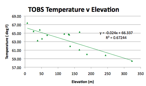Change in average Alabama temperature as a function of the elevation of the observing station.

The final correlation is with population, and there is not a really broad distribution of population around the stations., so that when this is included with the other variations, gives a poor correlation in the state with a 5-year average for temperature. (The correlation is, oddly, in this state better over longer periods).

Correlation of Alabama temperatures with the population of the community surrounding the station.

And that leaves the final check, between the raw data and that which has been modified to give the official USHCN numbers. The plot is the official temperature minus the raw temperature averages.


Let me throw in one final fact, just glancing at Chiefio’s site, he has a post up on relative humidity in which he quotes as follows:

As an average, the International Civil Aviation Organization (ICAO) defines an international standard atmosphere (ISA) with a temperature lapse rate of 6.49 K(°C)/1,000 m (3.56 °F or 1.98 K(°C)/1,000 Ft) from sea level to 11 km (36,090 ft). From 11 km (36,090 ft or 6.8 mi) up to 20 km (65,620 ft or 12.4 mi), the constant temperature is −56.5 °C (−69.7 °F), which is the lowest assumed temperature in the ISA.

Since I am using meters for measuring elevation but degrees Fahrenheit for temperature, the gradient is thus officially 11.68 deg/1,000 m or 0.0117 deg/m. The rate that the data fits, as shown above, is 0.024 deg, or about twice the official rate. It will be interesting to test the actual data for the different states against this standard.

E.M. Smith (who writes as Chiefio) has some interesting points to make about the effects of humidity, which I haven’t even thought of looking at, but which might be an interesting place to go. Water vapor is, after all, as he notes, supposed to be a stronger GreenHouse Gas (GHG) than carbon dioxide, and yet more humid places may be cooler than those which are drier. (It just may not feel that way). Read the post, it is interesting!